How to Freeze a Row in Google Sheets – Quick Navigation Tip

This document provides a concise guide on how to freeze rows in Google Sheets. Freezing rows is useful for keeping certain rows visible while scrolling through your data.

If you want to keep certain rows visible while scrolling through your spreadsheet, you can freeze them using the "View" menu. This is especially useful for keeping headers in place as you navigate down the page.

Step-by-step instructions:

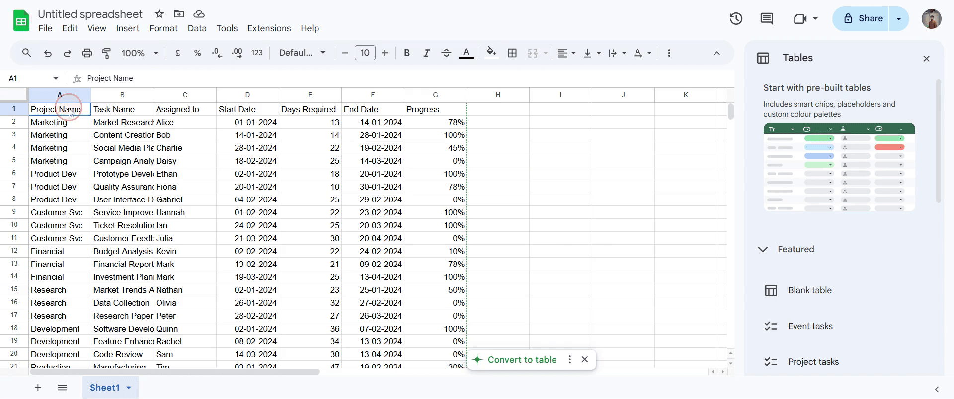
1. Open your Google Sheet:
Start by opening the spreadsheet where you want to freeze the rows.
2. Select the row(s):
Click on the row number on the left side to select the row you’d like to freeze. You can select more than one row if needed.
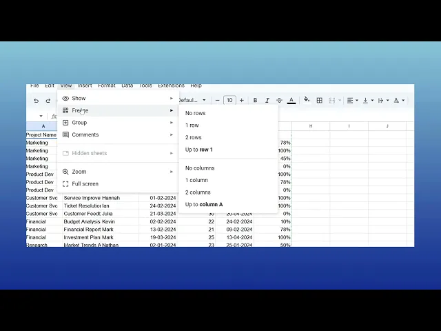
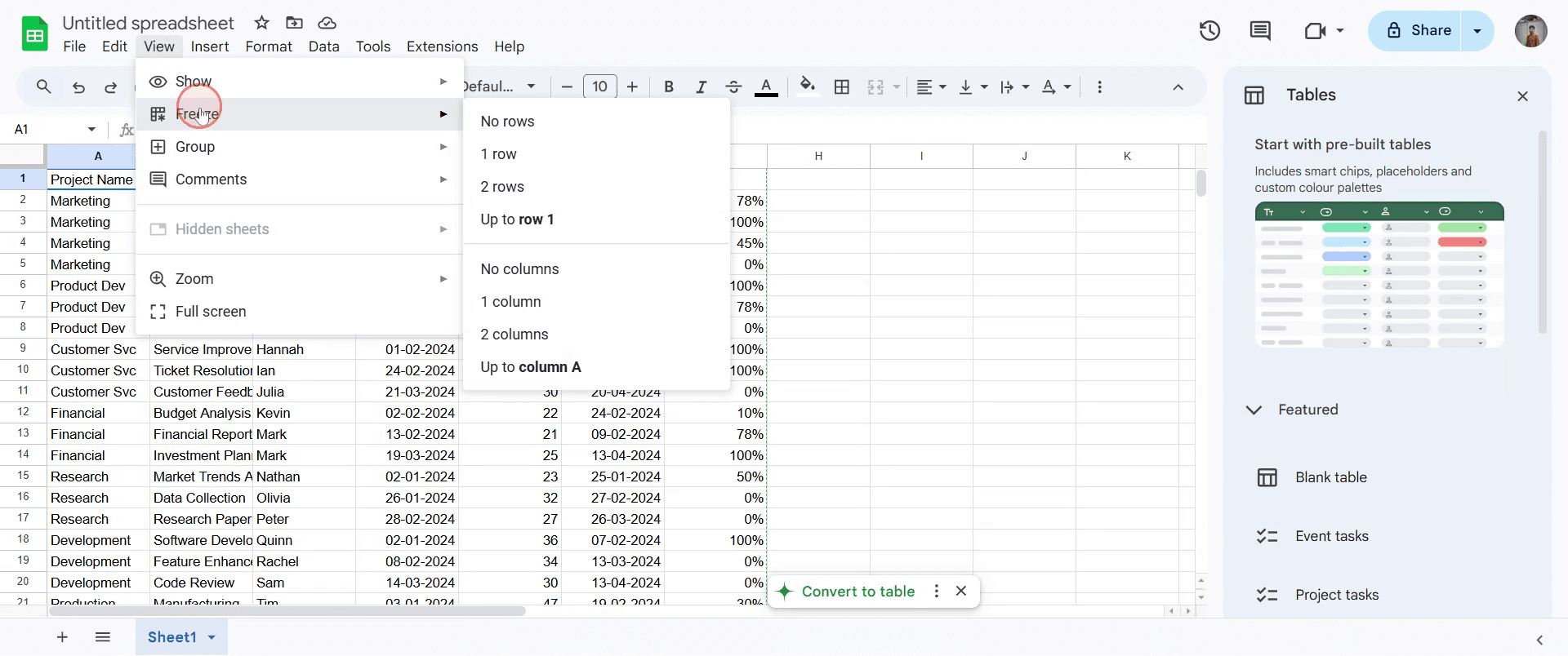
3. Open the “View” menu:
At the top of the page, click on "View" to open the dropdown menu.
4. Click on “Freeze”:
In the dropdown, hover over "Freeze" to see your freezing options.
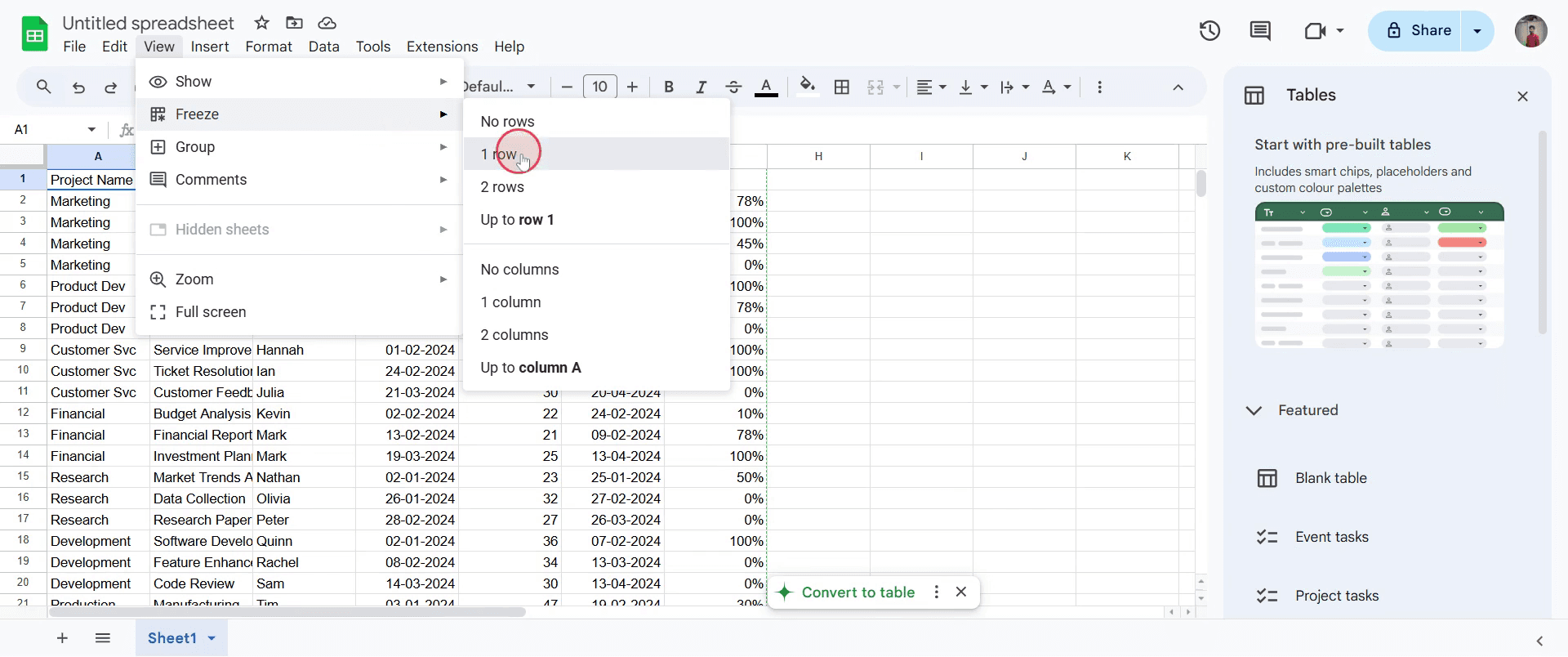
5. Choose how many rows to freeze:
Pick the number of rows you want to freeze like “1 row” to lock just the top row in place.
6. Done
The rows you selected will now stay fixed at the top of the sheet, even when you scroll down.

Step-by-Step Guide: How to Freeze a Row in Google Sheets

Step 1

Click on the desired row to select it.

Step 2

Go to View, select Freeze option

Step 3

A list of options will appear. Select the option that corresponds to the row you want to freeze.

Step 4

Verify that the entire row has been successfully frozen. This ensures that the selected row remains visible as you scroll through your sheet.

Pro-tips for freezing a row in a sheets

1. Freeze the top row to keep headers visible as you scroll through large spreadsheets for easy navigation.

2. Use the "Freeze Panes" option to freeze multiple rows at once, perfect for spreadsheets with a large header section.

3. Make sure to freeze only the necessary rows to keep your sheet efficient and avoid unnecessary screen space being taken up.

Common pitfalls & how to avoid them while Freezing rows in sheets

1. Forgetting to unfreeze rows when no longer needed can clutter your view remember to unfreeze if it's not necessary anymore.

2. Freezing too many rows can create confusion and reduce visibility freeze only the rows you need.

3. Not reviewing your spreadsheet's layout before freezing rows may lead to accidental freezing of irrelevant sections always double-check the rows you’re about to freeze.

Common FAQs on freeze a row in a sheets

1. What does the Freeze option do in Google Sheets?
   The Freeze option locks rows or columns so they stay visible while scrolling through the sheet.

2. How do I freeze a row or column in Google Sheets?
   Click View > Freeze, then choose to freeze one or more rows/columns.

3. Can I unfreeze rows or columns after freezing them?
   Yes, go to View > Freeze > No rows or No columns to remove the freeze.

4. How many rows or columns can I freeze?
   You can freeze up to any number of rows or columns from the top or left of the sheet.

5. Why is the Freeze option useful?
   It helps keep headers or important data visible while navigating large datasets

6. How to screen record on mac? 
   To screen record on a Mac, you can use Trupeer AI. It allows you to capture the entire screen and provides AI capabilities such as adding AI avatars, add voiceover, add zoom in and out in the video. With trupeer’s AI video translation feature, you can translate the video into 30+ languages. 

7. How to add an AI avatar to screen recording?
   To add an AI avatar to a screen recording, you'll need to use an AI screen recording tool. Trupeer AI is an AI screen recording tool, which helps you create videos with multiple avatars, also helps you in creating your own avatar for the video.

8. How to screen record on windows?
   To screen record on Windows, you can use the built-in Game Bar (Windows + G) or advanced AI tool like Trupeer AI for more advanced features such as AI avatars, voiceover, translation etc.

9. How to add voiceover to video?
   To add voiceover to videos, download trupeer ai chrome extension. Once signed up, upload your video with voice, choose the desired voiceover from trupeer and export your edited video. 

10. How do I Zoom in on a screen recording?
    To zoom in during a screen recording, use the zoom effects in Trupeer AI which allows you to zoom in and out at specific moments, enhancing the visual impact of your video content.