Como Criar uma Pauta no MS Excel

Aprenda a criar uma folha de notas profissional no Microsoft Excel. Tutorial passo a passo que aborda fórmulas, formatação e automatização para calcular facilmente os resultados dos alunos

Crie vídeos e documentação de produto impressionantes com IA

Este tutorial foi criado com o Trupeer em menos de 5 minutos

Crie gratuitamente

Aqui está um guia passo a passo:

1. Configure a estrutura básica:
Abra uma nova folha do Excel.
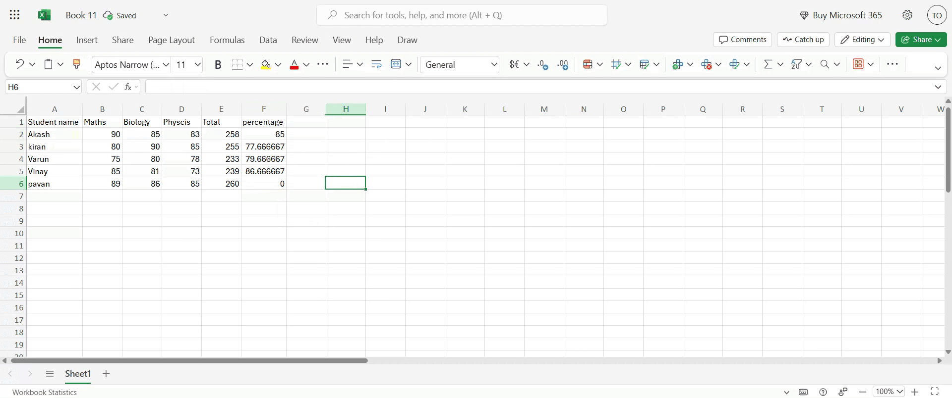
Crie colunas para N.º de aluno, Nome, Disciplina, etc., e Total, Percentagem, Classificação, Resultado (Aprovado/Reprovado).
Introduza os dados dos alunos e as notas nas respetivas colunas.
2. Calcule o total de pontos: Na coluna "Total", use a função SUM para somar as notas de cada aluno.
Por exemplo, se as notas de três disciplinas estiverem nas células C2, D2 e E2, a fórmula será =SUM(C2:E2).
Copie esta fórmula para baixo para calcular os totais de todos os alunos.
3. Calcule a Percentagem: Na coluna "Percentagem", divida o "Total" pelo número máximo possível de pontos e multiplique por 100.
Se o número máximo possível de pontos for 300, a fórmula será =(F2/300)*100 (assumindo que o Total está em F2).
Copie esta fórmula para baixo.
4. Atribua classificações: Use as funções IFS ou IF aninhadas para atribuir classificações com base na percentagem.
Por exemplo: =IFS(G2>=90,"A+",G2>=75,"A",G2>=60,"B",G2>=50,"C",G2>=35,"D",G2<35,"F") (assumindo que a Percentagem está em G2).
Isto atribui classificações com base em intervalos de percentagem.
5. Determine o estado de Aprovado/Reprovado: Use a função IF para verificar se a percentagem está acima do limite de aprovação (por exemplo, 35%).
Por exemplo: =IF(G2>=35,"Pass","Fail") (assumindo que a Percentagem está em G2).
6. Aplique Formatação Condicional: Selecione as células da coluna "Resultado".
Vá para Base > Formatação Condicional > Regras para Realçar Células > Texto que Contém.
Introduza "Fail" e escolha uma cor de preenchimento vermelha para os resultados reprovados.
Da mesma forma, pode realçar os resultados "Pass" com um preenchimento verde.
7. Melhorias opcionais: Pode adicionar uma coluna para classificar os alunos com base na sua pontuação total usando a função RANK.
Use a função VLOOKUP para apresentar informações adicionais do aluno a partir de outra folha ou tabela.
Use a função AVERAGE para calcular a média das notas dos alunos.

Guia Passo a Passo: Como Criar uma Pauta de Notas no MS Excel

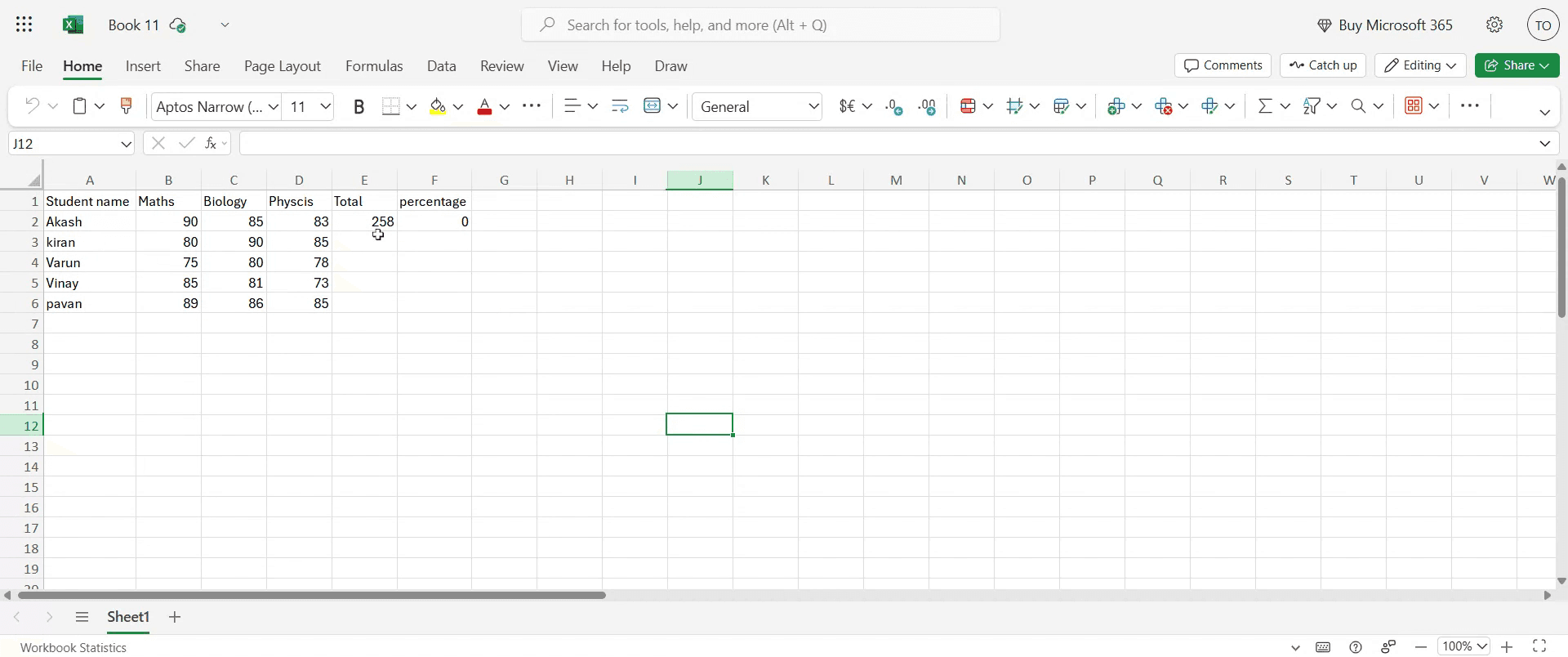
Passo 1

Depois de os dados terem sido introduzidos na folha, a nossa próxima tarefa é calcular o total de pontos.

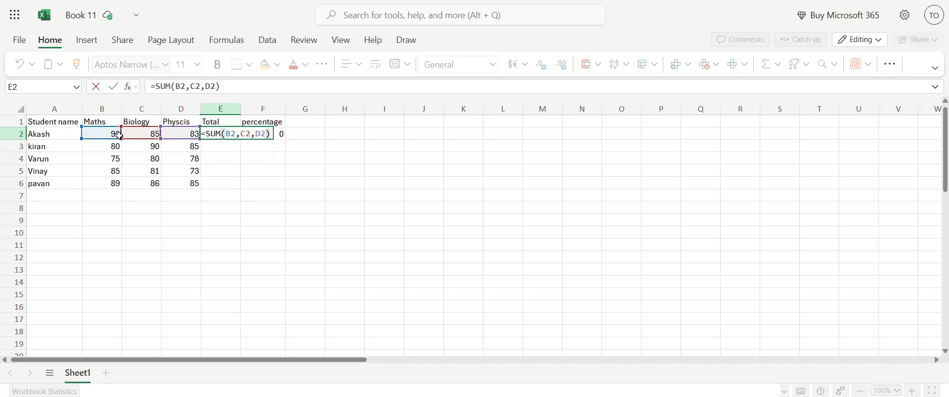
Once the details have been entered into the sheet, our next task is to calculate the total marks.

Passo 2

Selecione a célula desejada onde pretende que o total apareça. Introduza a fórmula neste formato: =SUM(cell2, cell3, cell4). Depois de inserir a fórmula, prima Enter. Agora verá o total de pontos calculado apresentado.

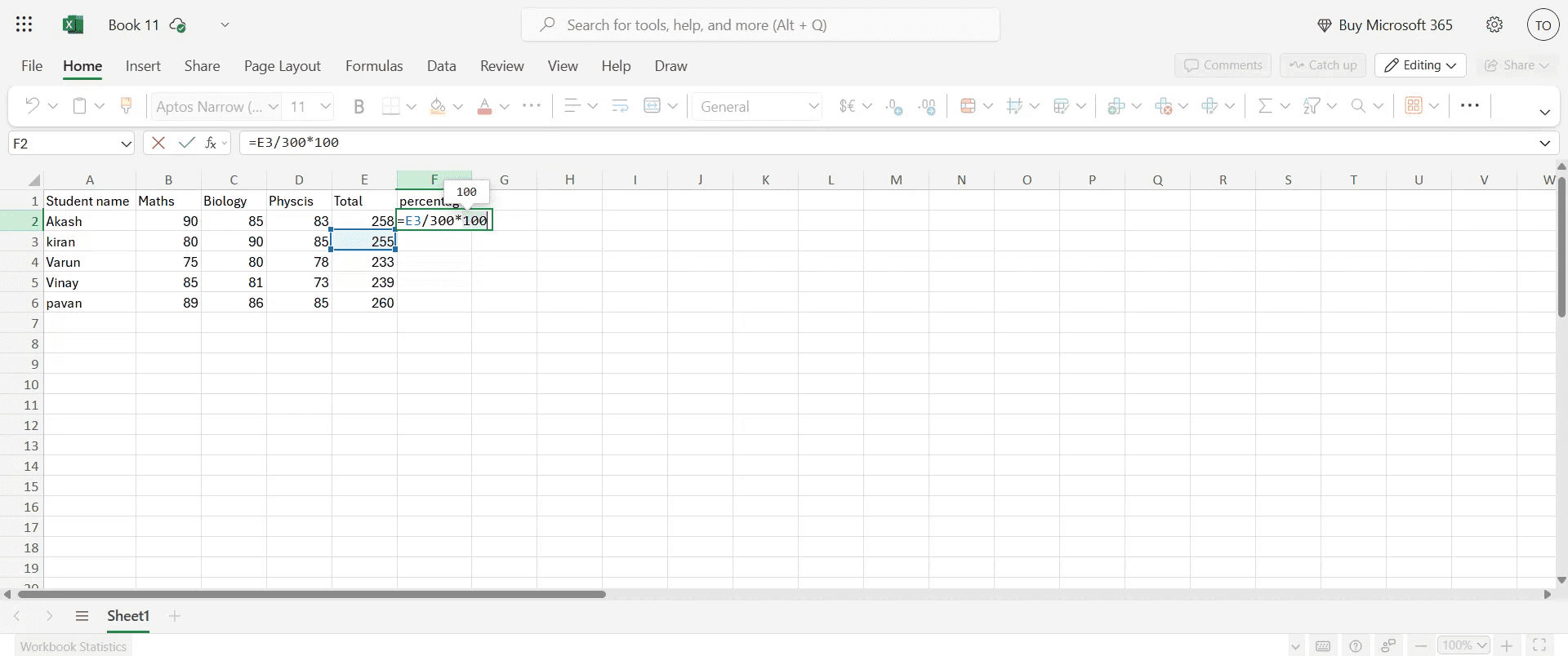
Select the desired cell where you want the total to appear. Enter the formula in this format: =SUM(cell2, cell3, cell4). After inputting the formula, press Enter. You will now see the calculated total marks displayed.

Passo 3

Para o cálculo da percentagem, selecione a célula da percentagem e introduza a fórmula: =(E3/TotalNumberOfSubjects)*100

For percentage calculation, select the percentage cell and input the formula: =(E3/TotalNumberOfSubjects)*100

Passo 4

Para aplicar o cálculo da percentagem a todas as disciplinas, use o método de arrastar e largar para estender a fórmula às células restantes.

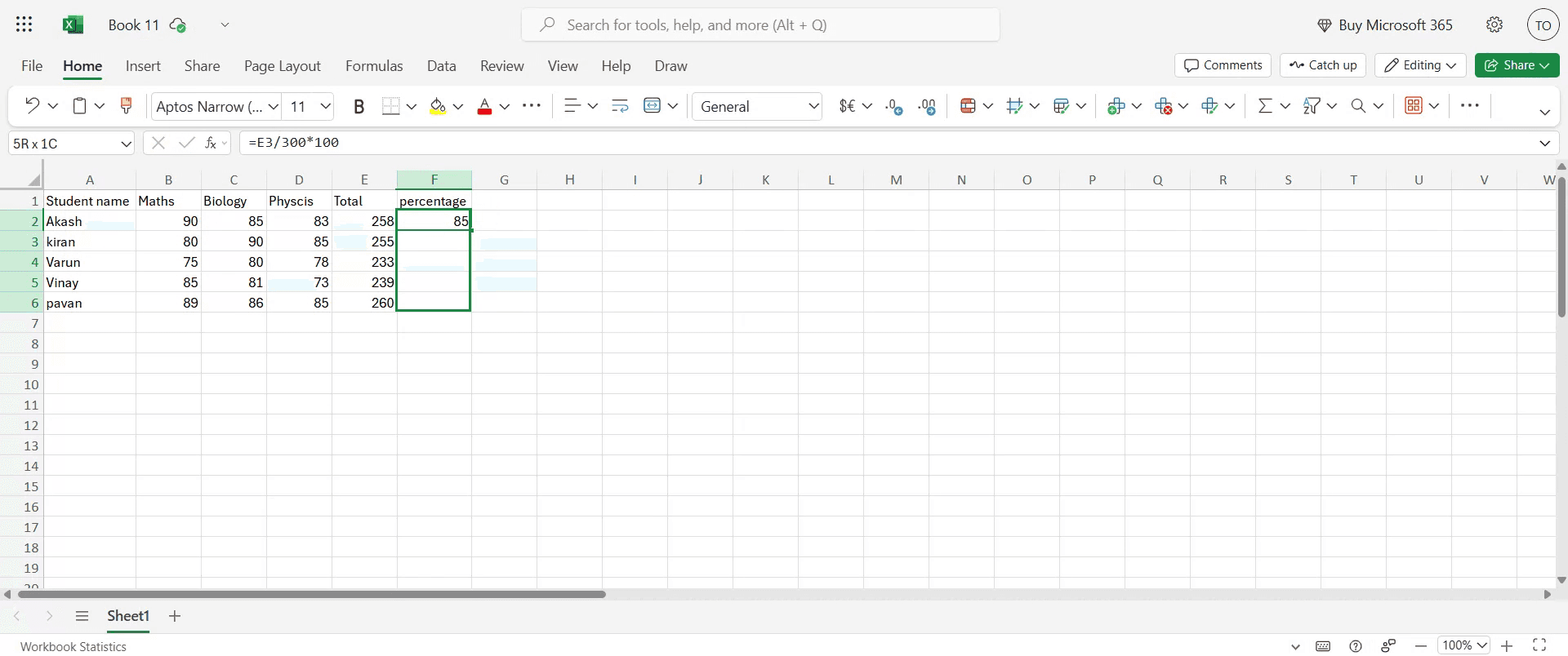
To apply the percentage calculation across all subjects, use the drag and drop method to extend the formula to the remaining cells.

Passo 5

Esta ação apresentará a percentagem de cada disciplina.

This action will display the percentage for each subject.

Dicas Profissionais para Criar uma Folha de Notas no Excel

Abra o Microsoft Excel
Inicie o Microsoft Excel e abra um novo livro em branco onde irá criar a sua folha de notas.
Defina os cabeçalhos das colunas
Na primeira linha, introduza cabeçalhos como Nº de aluno, Nome do aluno, Disciplina 1, Disciplina 2, Disciplina 3, Total, Média e Classificação.
Introduza dados de exemplo
Preencha os dados dos alunos e as classificações em cada disciplina. Mantenha os dados organizados para facilitar o cálculo dos totais e das médias.
Calcule a soma das notas
Na coluna Total, use uma fórmula como =SUM(C2:E2) se as notas das disciplinas estiverem nas colunas C, D e E. Arraste a fórmula para baixo para a aplicar a todas as linhas.
Calcule a média das notas
Na coluna Média, use uma fórmula como =AVERAGE(C2:E2) para calcular a média das notas de cada aluno.
Adicione um sistema de classificação
Na coluna Classificação, use uma fórmula IF aninhada como:
=IF(F2>=90, "A+", IF(F2>=75, "A", IF(F2>=60, "B", IF(F2>=40, "C", "F"))))
Isto atribui classificações com base na média ou no total das notas.

Erros Comuns e Como Evitá-los

Intervalos de fórmula incorretos
Certifique-se de que as suas fórmulas (como SUM ou AVERAGE) incluem as células corretas. Erros nas referências de células podem resultar em totais ou médias incorretos.
Esquecer-se de copiar as fórmulas para baixo
Depois de inserir fórmulas numa linha, arraste-as para baixo para as aplicar a todos os alunos. Caso contrário, apenas uma linha será calculada.
Substituir células com fórmulas
Bloqueie as colunas com fórmulas ou use a proteção de células para evitar que sejam substituídas acidentalmente por utilizadores que introduzem dados.
Não padronizar a lógica de classificação
Certifique-se de que o seu sistema de classificação é consistente e reflete a política da sua instituição. Reveja cuidadosamente a lógica utilizada nas instruções IF.
Ignorar a formatação
Uma folha simples pode ser difícil de ler. Use bordas, cabeçalhos em negrito e codificação por cores para tornar a folha de notas visualmente organizada.

Perguntas frequentes comuns sobre a criação de uma pauta de notas no Excel

Como calculo a classificação total no Excel?
Use =SUM(cell1:cellN) para somar as notas de várias disciplinas. Por exemplo, =SUM(C2:E2) adiciona as notas de três disciplinas.
O Excel pode atribuir classificações automaticamente?
Sim, usando fórmulas IF ou IF aninhadas, pode atribuir classificações com base nas notas ou médias.
Como posso garantir que as minhas fórmulas não são apagadas?
Proteja a folha indo a Rever → Proteger Folha e bloqueie as células que contêm fórmulas.
Existe uma forma de destacar os alunos que chumbaram?
Sim, use Formatação Condicional para destacar linhas em que a classificação é "F" ou em que a média esteja abaixo de um determinado limite.
Posso reutilizar o design da minha pauta de notas?
Sim, depois de configurar a sua primeira pauta de notas, guarde-a como um Modelo do Excel (*.xltx) para poder reutilizar a estrutura com novos dados.
Como gravar o ecrã no Mac?
Para gravar o ecrã num Mac, pode usar o Trupeer AI. Permite capturar o ecrã inteiro e fornece capacidades de IA como adicionar avatares de IA, adicionar narração e aplicar zoom in and out no vídeo. Com a funcionalidade de tradução de vídeo por IA da trupeer, pode traduzir o vídeo para mais de 30 idiomas.
Como adicionar um avatar de IA a uma gravação de ecrã?
Para adicionar um avatar de IA a uma gravação de ecrã, terá de usar uma ferramenta de gravação de ecrã com IA. Trupeer AI é uma ferramenta de gravação de ecrã com IA, que ajuda a criar vídeos com vários avatares e também ajuda a criar o seu próprio avatar para o vídeo.
Como gravar o ecrã no Windows?
Para gravar o ecrã no Windows, pode usar a Game Bar integrada (Windows + G) ou uma ferramenta avançada de IA como o Trupeer AI para funcionalidades mais avançadas, como avatares de IA, narração, tradução, etc.
Como adicionar narração a um vídeo?
Para adicionar narração a vídeos, descarregue a extensão Chrome do trupeer ai. Depois de se registar, carregue o seu vídeo com voz, escolha
a narração pretendida do trupeer e exporte o seu vídeo editado.
Como faço zoom numa gravação de ecrã?
Para aplicar zoom durante uma gravação de ecrã, use os efeitos de zoom no Trupeer AI, que permitem aproximar e afastar em momentos específicos, melhorando o impacto visual do conteúdo do seu vídeo.