如何在 MS Excel 中创建成绩单

以下是分步指南：

1. 设置基本结构：
打开一个新的Excel 工作表。 
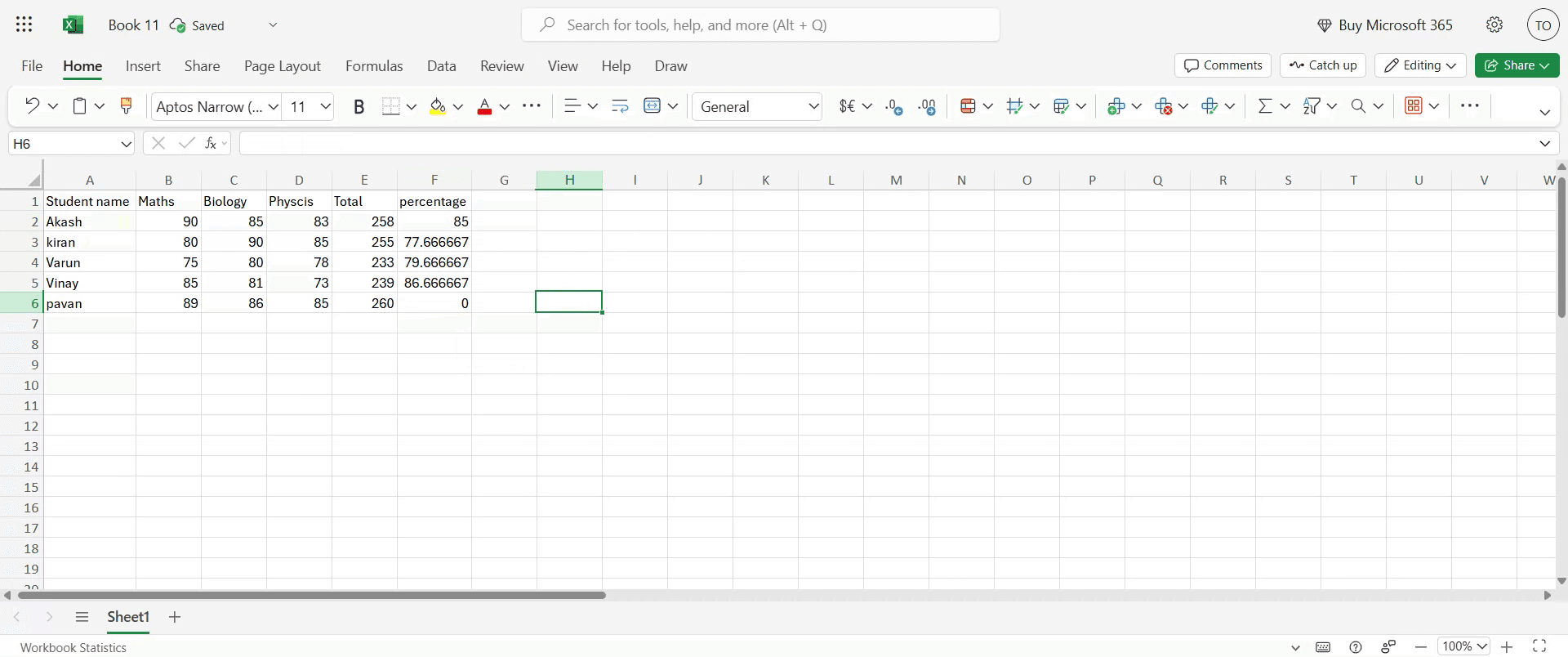
创建学号、姓名、科目等以及总分、百分比、等级、结果（通过/失败）的列。 
在相应的列中输入学生详细信息和分数。 
2. 计算总分：在“总分”列中，使用 SUM 函数将每个学生的分数相加。
例如，如果三个科目的分数分别在单元格 C2、D2 和 E2 中，则公式为 =SUM(C2:E2)。 
向下复制此公式，以计算所有学生的总分。 
3. 计算百分比：在“百分比”列中，将“总分”除以可获得的最高分，然后乘以 100。 
例如，如果最高分为 300，则公式为 =(F2/300)*100（假设总分在 F2 中）。 
向下复制此公式。 
4. 分配等级：使用 IFS 或嵌套 IF 函数根据百分比分配等级。 
例如：=IFS(G2>=90,"A+",G2>=75,"A",G2>=60,"B",G2>=50,"C",G2>=35,"D",G2<35,"F")（假设百分比在 G2 中）。 
这会根据百分比范围分配等级。
5. 确定通过/失败状态： 使用 IF 函数检查百分比是否高于及格阈值（例如 35%）。 
例如：=IF(G2>=35,"Pass","Fail")（假设百分比在 G2 中）。 
6. 应用条件格式：选择“结果”列中的单元格。 
转到 开始 > 条件格式 > 突出显示单元格规则 > 包含文本。 
输入“Fail”，并为不及格结果选择红色填充颜色。 
同样，你也可以为“Pass”结果使用绿色填充进行突出显示。 
7. 可选增强：你可以使用 RANK 函数根据学生的总分添加一个排名列。 
使用 VLOOKUP 函数从其他工作表或表格中显示额外的学生信息。 
使用 AVERAGE 函数计算学生的平均分。 

分步指南：如何在 MS Excel 中创建成绩单

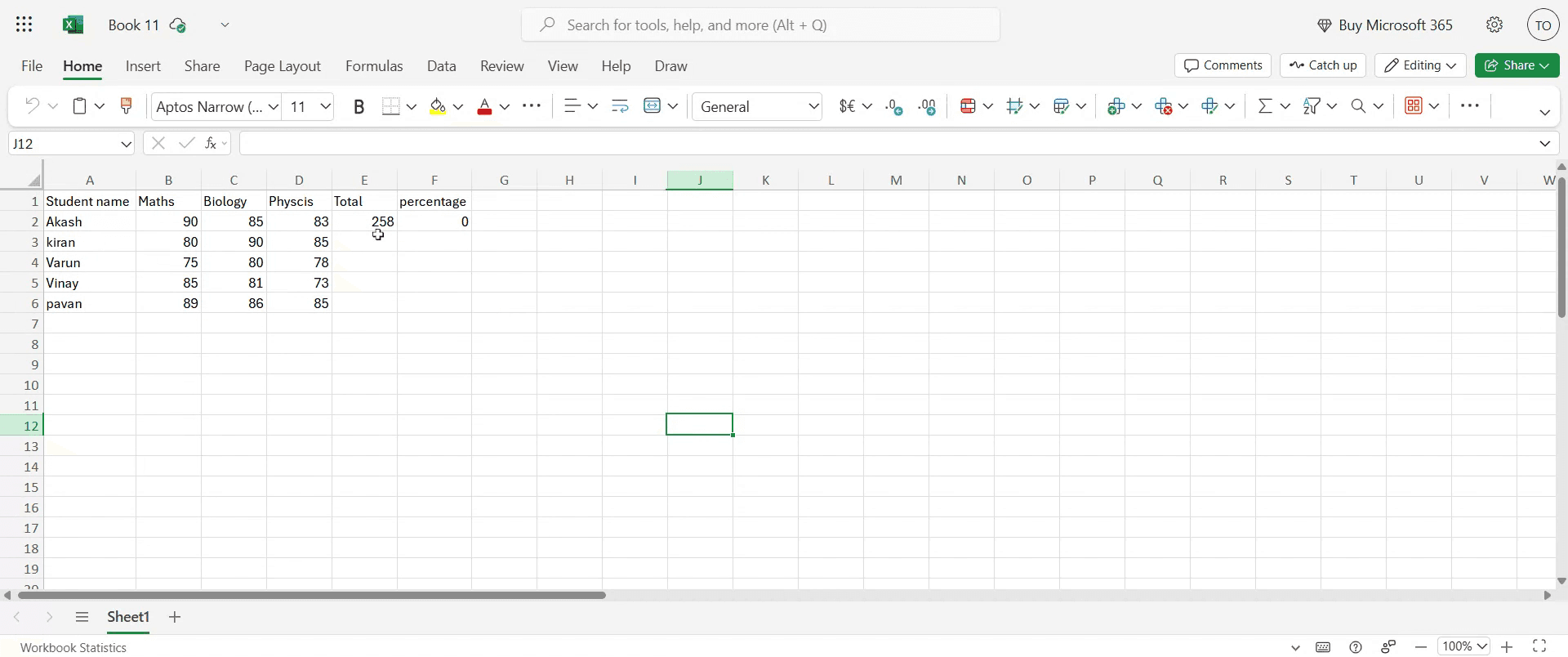
步骤 1

一旦详细信息已输入到工作表中，我们的下一步任务就是计算总分。

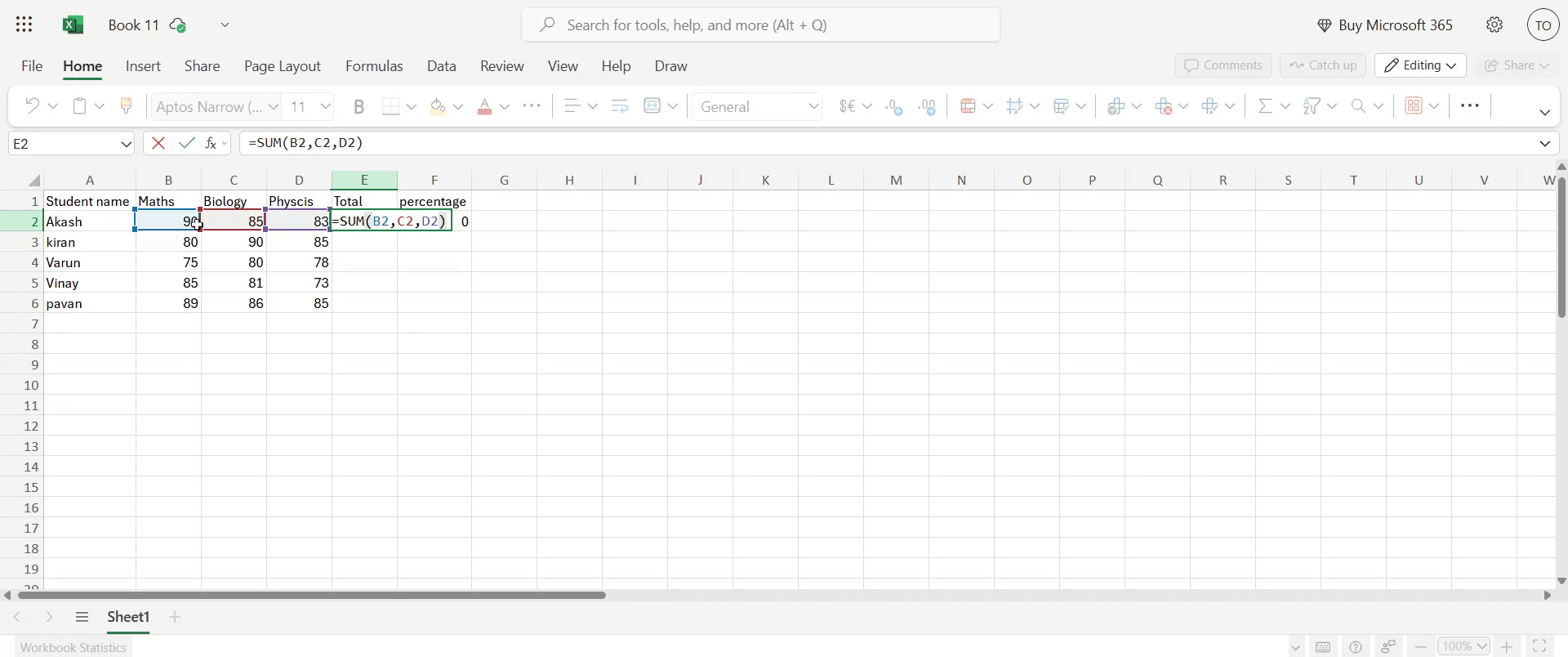
步骤 2

选择你希望显示总分的目标单元格。按照以下格式输入公式：=SUM(cell2, cell3, cell4)。输入公式后，按 Enter。你现在将看到计算出的总分显示出来。

步骤 3

对于百分比计算，选择百分比单元格并输入公式：=(E3/TotalNumberOfSubjects)*100

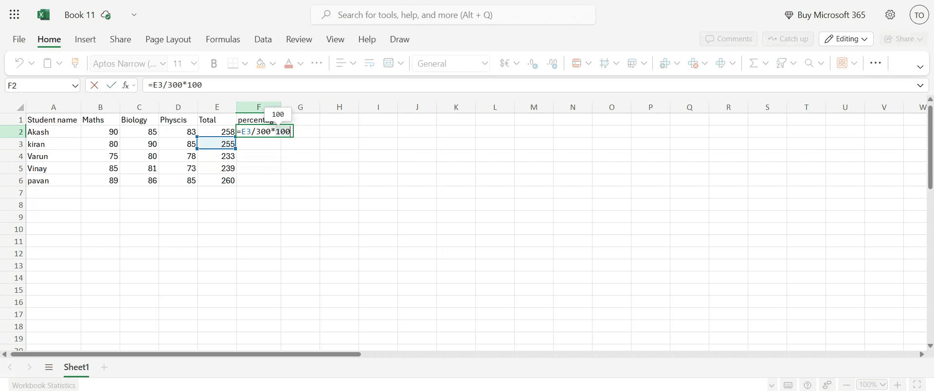
步骤 4

要将百分比计算应用到所有科目，请使用拖放方法将公式扩展到其余单元格。

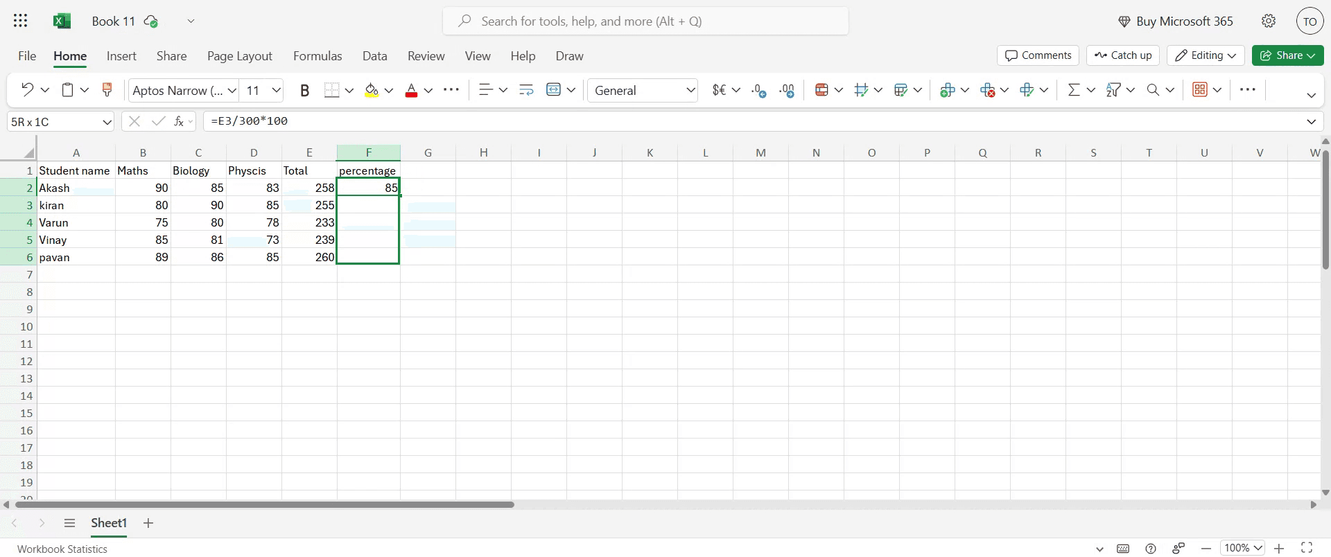
步骤 5

此操作将显示每个科目的百分比。